Current World Environment

Introduction

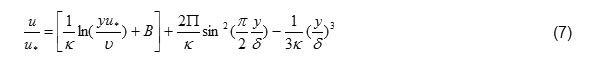
Experimental observations show that all velocity profiles in a turbulent shear flow (like Flow in open channels and pressure) divided in to parts (areas) on a straight line. The Disturbances internal area is affected with floor directly and external area is affected by shear stress and floor indirectly. The internal part divided three regions slow layer, middle layer and overlapping layer. While the change in internal part to external area is gradual, the overlapping layer is account the external part. Then the external part composes two areas overlapping layer and the Uplift layer (Circular movement’s part or wake).the figure 1 illustrated the Classification of these areas.

Many studies performed the velocity distribution in numerically and experimentally and presented different relationships yet. First, the research introduces the validity relationship and then, analyses the relationships and use the experimental data’s too. The best relationship Will be introduced by use the statistical analyses.

The most famous relation is provided for the estimated velocity distribution, logarithm distribution. Theodore van Karman used the logarithm distribution for the first time. The distribution is as follows:

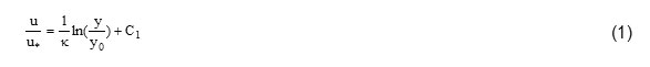
In relation. U Velocity at depth y,u/ Shear rate, fixed van Karman k,(for clean water equal ./41),y the depth is occur zero velocity.in the turn up maximum flow velocity, Logarithmic distribution is written as follows:

In the relation, δ is the height of maximum speed Unix. The simple relation and also the low number of variables considered the advantages of distribution. Although the most of relation of transmission of Sediment develop based on Logarithmic distribution. The logarithm law is valid to all of the internal area except near the channel floor, but the external part would be deviation from the experimental data’s. vernon , (Einstein and Chien,1955), (Venoni and nomicos ,1960), (elata and aypen, 1961) showed the logarithm law is valid in total flow.in the paper, with consider the fixed amount of van karman is equal 0/4 in throughout the depth of   flow and analyzed the velocity distribution.

The disadvantages of the distribution can noted the large of errors in Speed estimation in external part ((2/0y/h>),in this part ,Logarithmic distribution distracted the experimental data’s significantly .ever this deviation by the fixed van-karman or Cannot modify add additional fixed to Logarithmic law .venoni claims that the  Wide channels(5b/h>) and Central line speed  channel occurs surface water and Logarithmic law can use throughout Flow depth. But Normally, Narrow channels (5b/h<) occurs in below the water surface and Logarithmic distribution Will be applied only the internal area.

This distribution is not valid in the close the wall .also in the close the edge of the boundary layer was distance from experimental data’s. Nevertheless, this relation use all flat plate turbulent boundary layer, because that in the distribution velocity shape related to Local shear stress, is very helpful.

(Yang and Colleagues,2004) modified Logarithmic distribution by analyses nayver stokes rinolda equation and assuming a parabolic distribution for Eddy viscosity. They pay attention to effect on channel in velocity flow. The modified Logarithmic distribution is as follows:

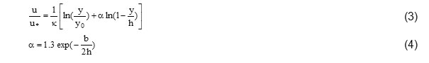
In this relation b is Channel width. A=0the above equation would be Logarithmic distribution.

(Coles,1956) was analyzed the velocity wind distribution in Dimensional low and add wake function to velocity Logarithmic distribution, the below relation is developed to estimate velocity for internal and external parts. This distribution is famous the wake law And are as follows:

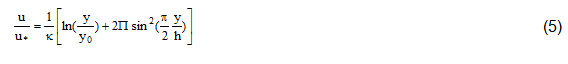
In this relation, Π is Coles coefficient or wake coefficient estimated with uses experimental data’s that is based on (Guo and julien,2008) opinions, because there is not valid relation to calculate. Properties of distribution is applied only the central part and it is not valid the flows occurs in the below layer by maximum speed. Maximum speed in the below layer occurs Channels by 5b/h< due of Strong shear stress near the wall and the occurrence of secondary flow. The case of Logarithmic law and wake law can’t be accurate estimation of speed in the near free layer in out region.

Nevertheless secondary flow and Occurrence the maximum speed in the below layer water, the wake law cannot be estimate the speed during the three-dimensional in open channels. Add wake function to modified Logarithmic law, proposed the following equation (modified Logarithmic distribution and wake):

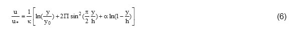
Guo and Julien modified the wake law that known the modified Logarithmic distribution and wake:

(Keulegan,1938) introduced parabolic distribution in his article and explained this distribution with experimental data’s is suggested by bazin. Parabolic distribution as follows:

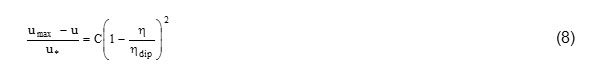
In the relation, c is a Numeric constant and determine to using experimental data’s, η Depth of the seabed (y/h), ηdip=yumax/h that yumax is accrued Maximum speed depth in umax, this distribution is applied throughout the Flow depth in narrow channels (5≥b/h) and the central part in External area. (Vedula and Rao,1985) concluded The point then is practical in parabolic distribution for Containing the suspended sediment inis  domain η=0/2 to η=0/3 and also illustrated the c parameter on This intersection. (Sarma et al.,2000) check out the Limitations and the credit of parabolic law. They claim Laboratory studies that the maximum in focus is while the maximum speed accurate in the water layer, Η=0/5 and the amount of maximum speed decreases in the water below layer. Also, they show that both of Logarithmic law and parabolic law are valid in Internal and external border areas and Velocity at this point is unique.

Materials and Methods

In the research uses the Reliable experimental data’s related to (Venoni,1946) and (Einstein,1955), to survey accuracy of each equation and determine the best equation. The experimental data’s is reliable data’s and most researchers use it to evaluate equations. These experiments performed in a flume width85/0 and 0/307 meter.

The main statistical indicators like the mean error (AE), least square root error (RMSE) and the regression coefficient (2R) is applied for Determine the best equation, to calculate each of these indicators is used the following relationships:

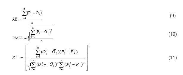
In this relation pi is the calculated values, Oi is measured values, in the number of samples and Ō the average value measured. Positive and negative values of AE Represents the Estimated at more than and less than the actual value, in order. The value of this index is lower; indicate the reliability of the equation. The amount of RMSE is always positive and approaching zero, Examined the relationship between increased. The amount of RMSE states the estimated error in the entire curve.

Results and Discussion

In the figure 2, is plotted the logarithmic velocity distribution (solid line) by experimental data’s. in this picture can be seen the changes in local area is more than the external part.

In the figure 3. Modified logarithmic distribution (the equation 1) compared with experimental data’s. Also, this distribution acts similar the logarithmic distribution. Given the Modified logarithmic distribution is intended effect of channel on the velocity distribution and due the figure can be concluded that the channel dimensions are not effect to the results. Comparison of the wake distribution (equation 2) illustrate in figure 4 by experimental data’s. The wake distribution estimates a month velocity in this picture. Also, this distribution estimates a month velocity in the inner and external areas.

Also, in the figure 5. The calculated values by modified logarithmic distribution –wake (equation 6) Compared Laboratory values

In the figure 6, is plotted the calculated values of the velocity parabolic distribution (equation 8) in contrast, laboratory values. As can be seen this distribution only can be estimate Speed values in the external area and Cleary, Distracted the experimental data’s in the local area.

To determine the velocity distribution equation indices was calculated score to each equation. In the table 1 presented The values of these parameters. It can be seen For all statistical based on Examined, wake distribution Relative superiority Compared to other equations. In the other hand, Parabolic distribution is less accurate in this equation. Of course, it must talk that Parabolic distribution is applied only the external area and occurs the maximum speed in below water level. Wake distribution well estimated Speed values in the total depth flow (local and external areas).

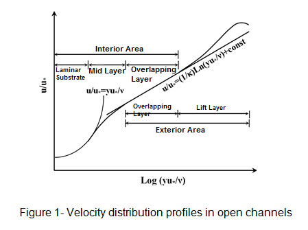Figure1: Velocity distribution profiles in open channels  Click here to View figure

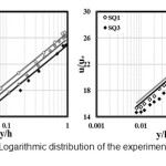Figure2: Logarithmic distribution of the experimental data’s   Click here to View figure

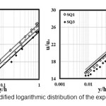Figure3: Modified logarithmic distribution of the experimental data’s  Click here to View figure

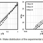Figure4: Wake distribution of the experimental data’s  Click here to View figure

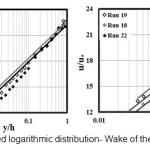Figure5: Modified logarithmic distribution- Wake of the experimental data’s  Click here to View figure

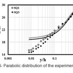Figure6: Parabolic distribution of the experimental data’s  Click here to View figure

Table 1: The results of the various equations with using statistical parameters

Conclusion

In the research check out for Calculate the velocity distribution in open channels by most developed equations. Such equations are investigated logarithmic distribution, modified logarithmic distribution, wake distribution- modified logarithmic distribution-wake and parabolic distribution. Calibration Each of these equations, is used the reliable experimental data’s. Then with using several statistical indicators, was select the best equation among equations. The results of equation illustrated that the wake distribution reasonably accurate estimates Speed values both of the local and external parts and Recommended using the equation in calculation relate to Depth distribution rate, on the other side, Parabolic distribution s less accurate and the use it will create large of errors in Calculation. Also, it has been said that the equation can only to estimate amount velocity in the outer region.

References

1. Chow, V.T. ,"Open Channel Hydraulics". McGraw-Hill Book Company, New York. (1959)
2. Coleman, N.L. ,"Effects of suspended sediment on the open-channel velocity distribution, Water Resources Research, 22 (10), 1377-1384 (1986)
3. Coles, D. ,"The law of the wake in the turbulent boundary layer", J. Fluid Mechanics, 1,191-226 (1956)
4. Einstein, H.A., and Chien, N. ,"Effects of heavy sediment concentrationnear the bed on velocity and sediment distribution", U. S. Army Corpsof Engineers, Missouri River Division Rep. 8. (1955)
5. Elata, C., and Ippen, A.T. ,"The dynamics of open channel flow with suspensions of neutrally buoyant particles", Technical Report No.45, Hydrodynamics Lab, MIT. (1961)
6. Guo, J, and Julien, P.Y. ,"Application of the Modified Log-Wake Law in Open-Channels", University of Nebraska- Lincoln, Civil Engineering Faculty Publications. (2008)
7. Keulegan, G.H ,"Laws of turbulent flow in open channels", J. Res., Nat.Bureau of Standards, 21, 707-741(1938)
8. Parker, G., and Coleman, N.L. "Simple model of sediment-laden flows", Journal of Hydraulic Engineering, ASCE, 112(5), 356-375 (1986)
9. Sarma, K.V.N., Prasad, B.V.R., and Sarma, A.K. ,"Detailed Study of Binary Law for Open Channels", Journal Hydraulic Engineering, 126(3), 210-214 (2000)
10. Schlichting, H. ,"Boundary Layer Theory", McGraw-Hill, New York. (1979)
11. Vanoni, V.A.,"Transportation of suspended sediment by water", Trans. ASCE,111, 67-133 (1946)
12. Vanoni, V.A., and Nomicos, G.N. ,"Resistance properties in sediment laden streams", Trans., ASCE, 125,1140-1175 (1960)
13. Vedula, S., and Rao, A.R. . "Bed Shear from Velocity Profiles: A New Approach", Journal Hydraulic Engineering, 111(1), 131-143 (1985)
14. Wang, X, and Qian, N. ,"Turbulence Characteristics of sediment-laden flow", J. Hydr. eng., 115(6), 781-799 (1989)
15. Wang, Z, Larsen, P. ,"Turbulent Structure of Water and Clay suspensions with Bed Load". J. Hydr. eng., 120(5), 577-601 (1992)
16. Yang, S.Q., Tan, S.K., and Lim, S.Y. "Velocity distribution and dip-phenomenon in smooth uniform open channel flows", J. Hydraulic Engineering, 130(12), 1179-1186 (2004)